


Latest Observation
2019.04.05 Fri
Spring has come.
Since last weekend, cherry blossoms have bloomed rapidly in the Kanto region, and the spring weather, having usual cycles of three cold days followed by four warm ones, has become.
Spring has come over Japan!
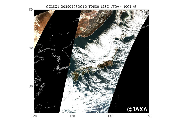
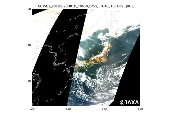
First, compare two color images around Japan taken by GCOM-C on January 3 and March 20, 2019 (see Figure 1). In the left winter image, you can see the typical winter clouds of cloud streaks, gathered by strong cold air blowing from the continent, and their disappearance in the right spring image. Instead, you can see that the typical early-spring haze caused by aerosols (fine particles suspended in the atmosphere) has begun to spread thinly over Japan. Also, the solar altitude is higher in March making the entire image brighter and indicating the arrival of spring.
Spring has come to plants!
Second, move Figure 2 and compare winter and spring images of an 8-day mean of the vegetation index, one of GCOM-C’s products that are commonly understandable physical quantities derived from observation data (left figures: early January 2019; right figures: late March 2019). The vegetation index is a metric for quantifying plant activity, with values closer to 1 indicating greater activity. You can see the expansion of the vegetation-covered area at Chikushi Plain in Kyushu in spring (center figures).
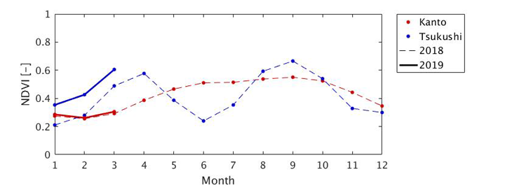
Third, see the seasonal changes in normalized difference vegetation index (NDVI) in the Chikushi Plain and the Kanto Plain (Figure 3). Spring plants grow faster and earlier in Chikushi Plain than in the Kanto Plain: You can see a rapid and early increase in NDVI in the Chikushi Plain and a slow and late increase in the Kanto Plain (compare the NDVI curves from January to April in Figure 3). You can also see such seasonality in Figure 2. The two peaks in NDVI on the Chikushi Plain represent double cropping.
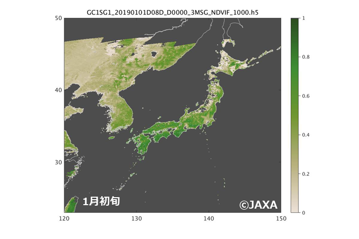
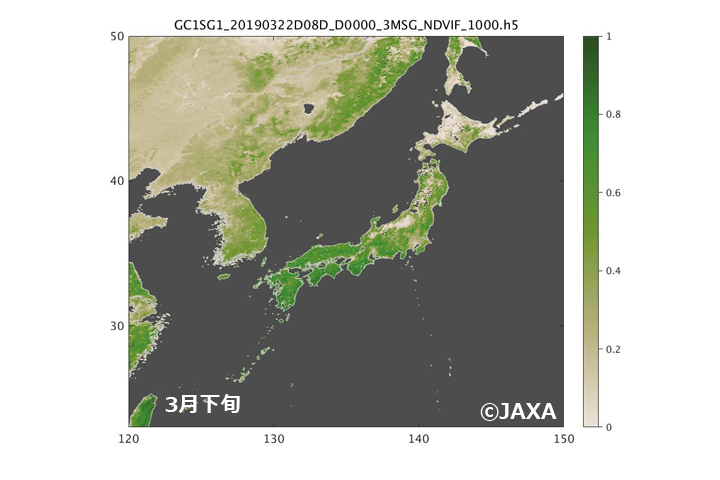


Figure 2. Eight-day mean of normalized difference vegetation index (NDVI) images observed by GCOM-C around Japan (left: January 1–8, 2019; right: March 22–29, 2019). The darker the green, the more active the vegetation. The center and bottom images are enlarged images of the Kyushu and Kanto regions.
Spring has come to sea surface temperatures!
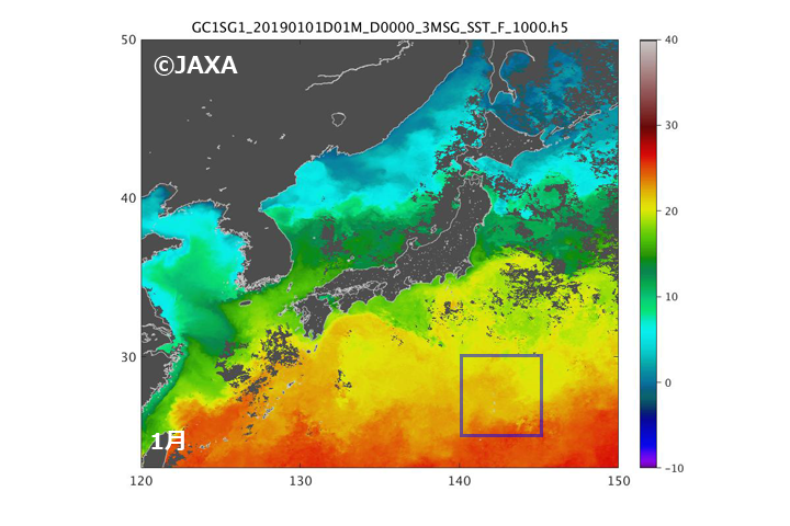
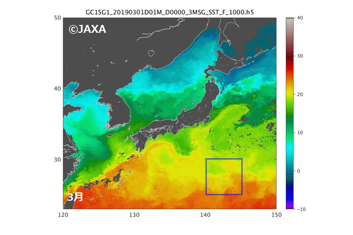
Fourth, move Figure 4 and compare the monthly mean images of GCOM-C sea surface temperature products (left: January 2019, right: March 2019). Generally, the air temperature gradually rises with the arrival of spring. In contrast, the sea surface temperature decreases in March compared to January. (In the right image, you can see a large green area corresponding to lower temperatures between 10 and 20 degrees Celsius.)
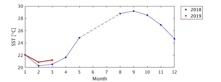
Seasonal changes in sea surface temperature lag behind changes in air temperature by one to two months according to the water’s larger heat capacity than air (it is more difficult to heat up and cool down). Figure 5 shows the seasonal changes in the monthly mean of sea surface temperature last year (2018) and this year (2019) in the area surrounded by a blue square in Figure 4.
The monthly mean of sea surface temperatures in 2018, with the lowest values in February and March and highest in September (see Figure 5). Based on seasonal changes in 2018 and the past, sea surface temperatures will rise from now (April) through September.
Spring has come to the sea!
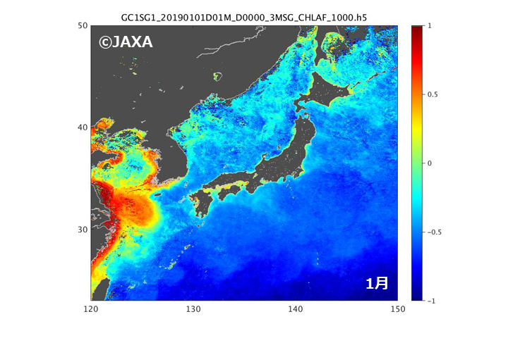
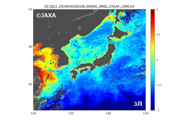
Fifth, move Figure 6 and compare the distribution of chlorophyll-a concentration in the sea observed by GCOM-C in January and March 2019 (Figure 6). Chlorophyll-a indicates the biomass of phytoplankton, which serves as food for marine life, including zooplankton. With the spring arrival, chlorophyll-a concentration in the Sea of Japan increases.
Similar to land, the timing of spring arrival in the sea has a spatial dependency. Spring blooms (the increase in phytoplankton) have already occurred in the Sea of Japan south of 40°N, not in further north areas. Chlorophyll-a concentrations usually increase at the coast of Hokkaido around April and May and in the Sea of Okhotsk from June with the spring arrival.
As for the spring increase of phytoplankton, see this also.
Spring has come to the world of snow and ice!
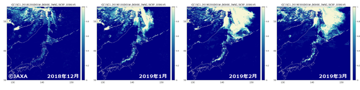
Sixth, compare the distribution of sea ice and snow cover (monthly statistics) observed by GCOM-C from December 2018 to March 2019 (Figure 7). The white denotes areas entirely covered with snow and ice in a month, while the light blue to blue denotes a decrease in the ratio of snow- and ice-covered periods.
As we introduced in a previous article, the ice originates from the Amur River in Russia and drifts south through the Sea of Okhotsk to reach Hokkaido in late January. The peak of the drift ice arrival was in February. Here, look at the right sub-figure. As you can see, the drift ice started disappearing (i.e., melting) in March: The white area changed to blue.
Most of the GCOM-C channels have a high spatial resolution of 250m. These allow long-term observation of physical quantities such as vegetation indices and sea surface temperatures with high resolution. It enables us to understand seasonal changes and anomalies everywhere in the world from space.
This year, no large-scale yellow sand that arrives at the Japanese archipelago on winds from the continent has yet been observed in March. However, yellow sand is usually observed in March and April.
GCOM-C has suitable channels to observe yellow sand: near-ultraviolet and thermal infrared wavelength channels with a high spatial resolution of 250m (see this article). These observations are expected to contribute to improving the accuracy of the Japan Meteorological Agency’s yellow sand forecasts.
Explanation of the Images
Figures 1, 2, 4, 6 and 7
| Satellite: | Global Change Observation Mission – Climate “SHIKISAI” (GCOM-C) |
|---|---|
| Sensor: | Second generation GLobal Imager (SGLI) |
| Date: | Figure 1: January 3, 2019 (left) and March 20, 2019 (right) Figure 2: January 1-8, 2019 (left) and March 22-29, 2019 (right) Figure 4: January 2019 (left) and March 2019 (right) Figure 6: January 2019 (left) and March 2019 (right) Figure 7: (From left to right) December 2018, January 2019, February 2019, March 2019 |
Related Links
Search by Year
Search by Categories


Tags
-
#Earthquake
-
#Land
-
#Satellite Data
-
#Aerosol
-
#Public Health
-
#GCOM-C
-
#Sea
-
#Atmosphere
-
#Ice
-
#Today's Earth
-
#Flood
-
#Water Cycle
-
#AW3D
-
#G-Portal
-
#EarthCARE
-
#Volcano
-
#Agriculture
-
#Himawari
-
#GHG
-
#GPM
-
#GOSAT
-
#Simulation
-
#GCOM-W
-
#Drought
-
#Fire
-
#Forest
-
#Cooperation
-
#Precipitation
-
#Typhoon
-
#DPR
-
#NEXRA
-
#ALOS
-
#GSMaP
-
#Climate Change
-
#Carbon Cycle
-
#API
-
#Humanities Sociology
-
#AMSR
-
#Land Use Land Cover
-
#Environmental issues
-
#Quick Report
Related Resources

Related Tags
Latest Observation Related Articles
-
 Latest Observation 2025.10.01 Wed [Quick Report] Hurricane Humberto “Eye” captured by EarthCARE satellite (Hakuryu)
 -
 Latest Observation 2025.02.28 Fri The world’s largest iceberg, A23a, may have run aground on the continental shelf of South Georgia:
The trajectory of iceberg A23a observed by “GCOM-W”, “ALOS-2” and “ALOS-4” -
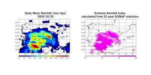 Latest Observation 2024.11.06 Wed [Quick Report] Heavy rainfalls in eastern Spain, as seen by the Global Satellite Mapping of Precipitation (GSMaP)
 -
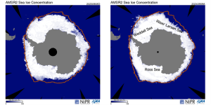 Latest Observation 2024.10.11 Fri Antarctic Winter Sea Ice Extent Second lowest in Satellite History
Stay Connected
